Research
Decoupled Neural Interfaces Using Synthetic Gradients
This post introduces some of our latest research in progressing the capabilities and training procedures of neural networks called Decoupled Neural Interfaces using Synthetic Gradients. This work gives us a way to allow neural networks to communicate, to learn to send messages between themselves, in a decoupled, scalable manner paving the way for multiple neural networks to communicate with each other or improving the long term temporal dependency of recurrent networks. This is achieved by using a model to approximate error gradients, rather than by computing error gradients explicitly with backpropagation. The rest of this post assumes some familiarity with neural networks and how to train them. If you’re new to this area we highly recommend Nando de Freitas lecture series on Youtube on deep learning and neural networks.
Neural networks and the problem of locking
If you consider any layer or module in a neural network, it can only be updated once all the subsequent modules of the network have been executed, and gradients have been backpropagated to it. For example look at this simple feed-forward network:
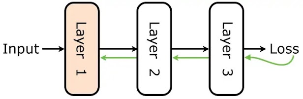
Here, after Layer 1 has processed the input, it can only be updated after the output activations (black lines) have been propagated through the rest of the network, generated a loss, and the error gradients (green lines) backpropagated through every layer until Layer 1 is reached. This sequence of operations means that Layer 1 has to wait for the forwards and backwards computation of Layer 2 and Layer 3 before it can update. Layer 1 is locked, coupled, to the rest of the network.
Why is this a problem? Clearly for a simple feed-forward network as depicted we don’t need to worry about this issue. But consider a complex system of multiple networks, acting in multiple environments at asynchronous and irregular timescales.
Or a big distributed network spread over multiple machines. Sometimes requiring all modules in a network to wait for all other modules to execute and backpropagate gradients is overly time consuming or even intractable. If we decouple the interfaces - the connections - between modules, every module can be updated independently, and is not locked to the rest of the network.
So, how can one decouple neural interfaces - that is decouple the connections between network modules - and still allow the modules to learn to interact? In this paper, we remove the reliance on backpropagation to get error gradients, and instead learn a parametric model which predicts what the gradients will be based upon only local information. We call these predicted gradients synthetic gradients.
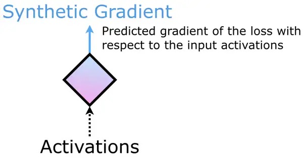
The synthetic gradient model takes in the activations from a module and produces what it predicts will be the error gradients - the gradient of the loss of the network with respect to the activations.
Going back to our simple feed-forward network example, if we have a synthetic gradient model we can do the following:
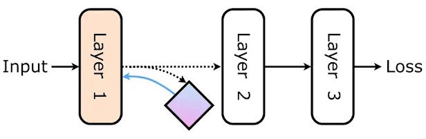
... and use the synthetic gradients (blue) to update Layer 1 before the rest of the network has even been executed.
The synthetic gradient model itself is trained to regress target gradients - these target gradients could be the true gradients backpropagated from the loss or other synthetic gradients which have been backpropagated from a further downstream synthetic gradient model.
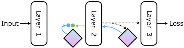
This mechanism is generic for a connection between any two modules, not just in a feed-forward network. The play-by-play working of this mechanism is shown below, where the change of colour of a module indicates an update to the weights of that module.
Using decoupled neural interfaces (DNI) therefore removes the locking of preceding modules to subsequent modules in a network. In experiments from the paper, we show we can train convolutional neural networks for CIFAR-10 image classification where every layer is decoupled using synthetic gradients to the same accuracy as using backpropagation. It’s important to recognise that DNI doesn’t magically allow networks to train without true gradient information. The true gradient information does percolate backwards through the network, but just slower and over many training iterations, through the losses of the synthetic gradient models. The synthetic gradient models approximate and smooth over the absence of true gradients.
A legitimate question at this point would be to ask how much computational complexity do these synthetic gradient models add - perhaps you would need a synthetic gradient model architecture that is as complex as the network itself. Quite surprisingly, the synthetic gradient models can be very simple. For feed-forward nets, we actually found out that even a single linear layer works well as a synthetic gradient model. Consequently it is both very easy to train and so produces synthetic gradients rapidly.
DNI can be applied to any generic neural network architecture, not just feed-forward networks. An interesting application is to recurrent neural networks (RNNs). An RNN has a recurrent core which is unrolled - repeatedly applied - to process sequential data. Ideally to train an RNN we would unroll the core over the whole sequence (which could be infinitely long), and use backpropagation through time (BPTT) to propagate error gradients backwards through the graph.
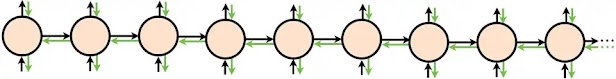
However in practice, we can only afford to unroll for a limited number of steps due to memory constraints and the need to actually compute an update to our core model frequently. This is called truncated backpropagation through time, and shown below for a truncation of three steps:
The change in colour of the core illustrates an update to the core, that the weights have been updated. In this example, truncated BPTT seems to address some issues with training - we can now update our core weights every three steps and only need three cores in memory. However, the fact that there is no backpropagation of error gradients over more than three steps means that the update to the core will not be directly influenced by errors made more than two steps in the future. This limits the temporal dependency that the RNN can learn to model.
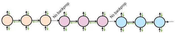
What if instead of doing no backpropagation between the boundary of BPTT we used DNI and produce synthetic gradients, which model what the error gradients of the future will be? We can incorporate a synthetic gradient model into the core so that at every time step, the RNN core produces not only the output but also the synthetic gradients. In this case, the synthetic gradients would be the predicted gradients of the all future losses with respect to the hidden state activation of the previous timestep. The synthetic gradients are only used at the boundaries of truncated BPTT where we would have had no gradients before.

This can be performed during training very efficiently - it merely requires us to keep an extra core in memory as illustrated below. Here a green dotted border indicates just computing gradients with respect to the input state, while a solid green border additionally computes gradients with respect to the core’s parameters.
By using DNI and synthetic gradients with an RNN, we are approximating doing backpropagation across an infinitely unrolled RNN. In practice, this results in RNNs which can model longer temporal dependencies. Here’s an example result showing this from the paper.
Penn Treebank test error during training (lower is better):

This graph shows the application of an RNN trained on next character prediction on Penn Treebank, a language modelling problem. On the y-axis the bits-per-character (BPC) is given, where smaller is better. The x-axis is the number of characters seen by the model as training progresses. The dotted blue, red and grey lines are RNNs trained with truncated BPTT, unrolled for 8 steps, 20 steps and 40 steps - the higher the number of steps the RNN is unrolled before performing backpropagation through time, the better the model is, but the slower it trains. When DNI is used on the RNN unrolled 8 steps (solid blue line) the RNN is able to capture the long term dependency of the 40-step model, but is trained twice as fast (both in terms of data and wall clock time on a regular desktop machine with a single GPU).
To reiterate, adding synthetic gradient models allows us to decouple the updates between two parts of a network. DNI can also be applied on hierarchical RNN models - system of two (or more) RNNs running at different timescales. As we show in the paper, DNI significantly improves the training speed of these models by enabling the update rate of higher level modules.
Hopefully from the explanations in this post, and a brief look at some of the experiments we report in the paper it is evident that it is possible to create decoupled neural interfaces. This is done by creating a synthetic gradient model which takes in local information and predicts what the error gradient will be. At a high level, this can be thought of as a communication protocol between two modules. One module sends a message (current activations), another one receives the message, and evaluates it using a model of utility (the synthetic gradient model). The model of utility allows the receiver to provide instant feedback (synthetic gradient) to the sender, rather than having to wait for the evaluation of the true utility of the message (via backpropagation). This framework can also be thought about from an error critic point of view [Werbos] and is similar in flavour to using a critic in reinforcement learning [Baxter].
These decoupled neural interfaces allow distributed training of networks, enhance the temporal dependency learnt with RNNs, and speed up hierarchical RNN systems. We’re excited to explore what the future holds for DNI, as we think this is going to be an important basis for opening up more modular, decoupled, and asynchronous model architectures. Finally, there are lots more details, tricks, and full experiments which you can find in the paper here.
Neural networks are the workhorse of many of the algorithms developed at DeepMind. For example, AlphaGo uses convolutional neural networks to evaluate board positions in the game of Go and DQNand Deep Reinforcement Learning algorithms use neural networks to choose actions to play at super-human level on video games.